An Example to Accelerate R with Rcpp and OpenMP: a Simulation Study of Survey with Systematic Non-responses
Result: Using
RcppwithOpenMPcan accelerate the simulation about 70 times inR.
This note uses a simple simulation study1 as an example to show that using Rcpp with OpenMP can significantly accelerate computation in R.
The simulation illustrates biases arising from systematic unit non-responses.
Specifically, I study biases in
- estimates of regression coefficients,
- the Horvitz-Thompson (HT) estimator and
- the variance estimator of the HT estimator.
Simulation
Simulation Setup
1. Population Generation
A bivariate fixed population \((X, Y)\) of size \(N = 1000\) comes from the following procedures:
- Generate the covariate \(X\) from \(U[0, 4]\).
- Generate the disturbance term \(e\) from \(N(0,1)\).
- The survey response variable \(Y = 1 + 2X + e\).
If a unit satisfy the condition \(-1 < y - x - 2 < 1\), then this unit is a response. Otherwise, the unit is a non-response.
The R code for generating the fixed population:
set.seed(123456)
N = 1000
x = runif(N, 0, 4)
e = rnorm(N, 0, 1)
y = 1 + 2*x + e
The R code to generate a vector of indices of responses.
tmp = y - x - 2
pop.response.index = which((tmp > -1) & (tmp < 1))
The response rate is about 40%.
2. Simulation Procedure
Repeat the following two steps \(R = 1000\) times.
-
Draw a 10%-sample (size \(n = 100\)) from the fixed population according to simple random sampling without replacement (SRSWOR).
-
Ignoring non-responses, I use only response units to
- fit a simple linear regression and record the two estimated coefficients,
- calculate the HT estimator ,
- estimate the variance of the HT estimator and
- record the number of responses.
Using these recorded statistics, I calculate the Monte-Carlo relative biases and the Monte-Carlo number of responses.
Simulation Results
The following data table summarize simulation results.
                     Full Response Non-response
rel.bias.intercept            6.33         71.4
rel.bias.slope               -1.51        -37.4
rel.bias.HT.mean            0.0268        -30.7
rel.bias.var.HT.mean        0.0932        -37.3
num.response                   100         40.2
Simulation Results:
If non-responses are ignored, the non-response biases are huge for estimated regression coefficients (intercept and slope), the HT estimator and the estimator of the variance of the HT estimator.
Simulation Programs
R only
- Variables setup:
n = 100 population = list( intercept = 1, slope = 2, mean = mean(y), var = (1 - n/N) * var(y) / n ) non.response = list( intercept = numeric(length=R), slope = numeric(length=R), HT.mean = numeric(length=R), var.HT.mean = numeric(length=R), num.response = numeric(length=R) ) - Helper function to record statistics from each replication:
SRSWOR = function(r, sample.x, sample.y, rt.lst) { model = lm(formula = "sample.y ~ sample.x") rt.lst$intercept[r] = as.numeric(model$coefficients[1]) rt.lst$slope[r] = as.numeric(model$coefficients[2]) rt.lst$HT.mean[r] = mean(sample.y) rt.lst$var.HT.mean[r] = (1 - length(sample.y)/N) * var(sample.y) / length(sample.y) rt.lst$num.response[r] = length(sample.y) return(rt.lst) } - Helper function to calculate Monte-Carlo statistics from the simulation:
cal.statistics = function(lst) { rel.bias.intercept = (mean(lst$intercept) - population$intercept) / population$intercept * 100 rel.bias.slope = (mean(lst$slope) - population$slope) / population$slope * 100 rel.bias.HT.mean = (mean(lst$HT.mean) - population$mean) / population$mean * 100 rel.bias.var.HT.mean = (mean(lst$var.HT.mean) - population$var) / population$var * 100 num.response = mean(lst$num.response) rt.lst = list( rel.bias.intercept = rel.bias.intercept, rel.bias.slope = rel.bias.slope, rel.bias.HT.mean = rel.bias.HT.mean, rel.bias.var.HT.mean = rel.bias.var.HT.mean, num.response = num.response) return(rt.lst) } - The function to run the simulation:
r.sim = function(R = 1000) {
  for (r in 1:R) {
      sample.index = sample(index, size = n, replace = FALSE)

      # SRSWOR with non-response
      sample.response.index = intersect(pop.response.index, sample.index)
      sample.y = y[sample.response.index]
      sample.x = x[sample.response.index]
      non.response = SRSWOR(r, sample.x, sample.y, non.response)
  }
  non.response.stat = cal.statistics(non.response)
  return(non.response.stat)
}
Rcpp
- The
C++function for simulation in the source filesimulation.cpp:// [[Rcpp::export()]] Rcpp::List simulation(const unsigned int R, const unsigned int sample_size, arma::vec y, arma::vec x, arma::uvec response_index) { // WARNING: indices for arrays in C++ starts from 0, // but those in R starts from 1 response_index = response_index - 1; const unsigned int N = y.n_rows; Simulation_results s(R, N, arma::mean(y)); for (unsigned int r = 0; r < R; ++r) { arma::uvec sample_index = arma::randperm<arma::uvec>(N, sample_size); arma::uvec sample_response_index = arma::intersect(response_index, sample_index); arma::vec sample_y = y.elem(sample_response_index); arma::vec sample_x = x.elem(sample_response_index); s.simulation(r, sample_x, sample_y); } s.compute_results(); return Rcpp::List::create( Rcpp::_["intercept"] = s.MC_intercept, Rcpp::_["slope"] = s.MC_slope, Rcpp::_["HT.mean"] = s.MC_HT_mean, Rcpp::_["var.HT.mean"] = s.MC_var_HT_mean, Rcpp::_["num.response"] = s.MC_num_response ); }Download the full
c++source file simulation.cpp. - We load the library
Rcppand theC++source file inR.library(Rcpp) sourceCpp("simulation.cpp")
Rcpp with OpenMP
-
Usually, when we run a program, the program is executed line by line (squentially). The above two (R only and Rcpp) are sequential programs.
-
Because each simulation replication does not affect the other, running iterations simultaneously instead of sequentially does not change the simulation outcome. Therefore, I use
OpenMPto assign each computer processor to run simulation replications in parallel to save computation time. This type of programming is called parallel programming. - The exhibit below explains the shorter runtime when using
OpenMP2.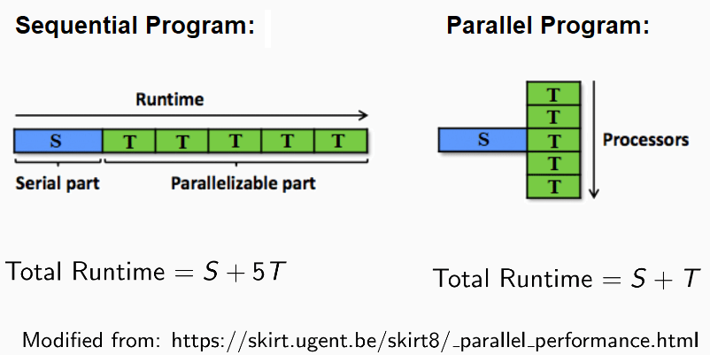
- The
C++function for simulation in the source filesimulation.cppuses 5 processors at the same time:// [[Rcpp::export()]] Rcpp::List simulation_p(const unsigned int R, const unsigned int sample_size, arma::vec y, arma::vec x, arma::uvec response_index) { // WARNING: indices for arrays in C++ starts from 0, // but those in R starts from 1 response_index = response_index - 1; const unsigned int N = y.n_rows; Simulation_results s(R, N, arma::mean(y)); omp_set_num_threads(5); # pragma omp parallel for for (unsigned int r = 0; r < R; ++r) { arma::uvec sample_index = arma::randperm<arma::uvec>(N, sample_size); arma::uvec sample_response_index = arma::intersect(response_index, sample_index); arma::vec sample_y = y.elem(sample_response_index); arma::vec sample_x = x.elem(sample_response_index); s.simulation(r, sample_x, sample_y); } s.compute_results(); return Rcpp::List::create( Rcpp::_["intercept"] = s.MC_intercept, Rcpp::_["slope"] = s.MC_slope, Rcpp::_["HT.mean"] = s.MC_HT_mean, Rcpp::_["var.HT.mean"] = s.MC_var_HT_mean, Rcpp::_["num.response"] = s.MC_num_response ); }Download the full
c++source file simulation.cpp. - We load the library
Rcppand theC++source file inR.library(Rcpp) Sys.setenv("PKG_CXXFLAGS" = "-fopenmp") Sys.setenv("PKG_LIBS" = "-fopenmp") sourceCpp("simulation.cpp")The two lines
Sys.setenv("PKG_CXXFLAGS" = "-fopenmp")andSys.setenv("PKG_LIBS" = "-fopenmp")are to flag the use ofOpenMPfor theg++compiler.
R Vs. Rcpp Vs. Rcpp with OpenMP: Rcpp with OpenMP Fastest
- Runtime comparison:
library(microbenchmark) microbenchmark( r = {r.sim()}, rcpp = {simulation(R = 1000, sample_size = 100, y = y, x = x, response_index = pop.response.index)}, rcpp2 = {simulation_p(R = 1000, sample_size = 100, y = y, x = x, response_index = pop.response.index)}, times = 100L )Output:
Unit: milliseconds expr min lq mean median uq max neval r 993.5976 1087.29510 1250.67629 1159.58185 1393.59430 2131.4919 100 rcpp 45.5461 48.05155 51.66997 51.06960 53.92465 67.7078 100 rcpp2 24.2971 25.74590 26.57889 26.39155 27.18675 31.1330 100Result: Using
RcppwithOpenMPcan accelerate the simulation about 70 (\(2131.4919 / 31.1330 \approx 68.5\)) times inR.
Footnote
-
The simulation setup comes from Yap (2020). ↩
-
The
OpenMPsupports shared-memory multi-platform parallel programming in Fortran, C and C++. For details, refer to the official page for OpenMP. ↩